Weekly Work Commitments Calendar

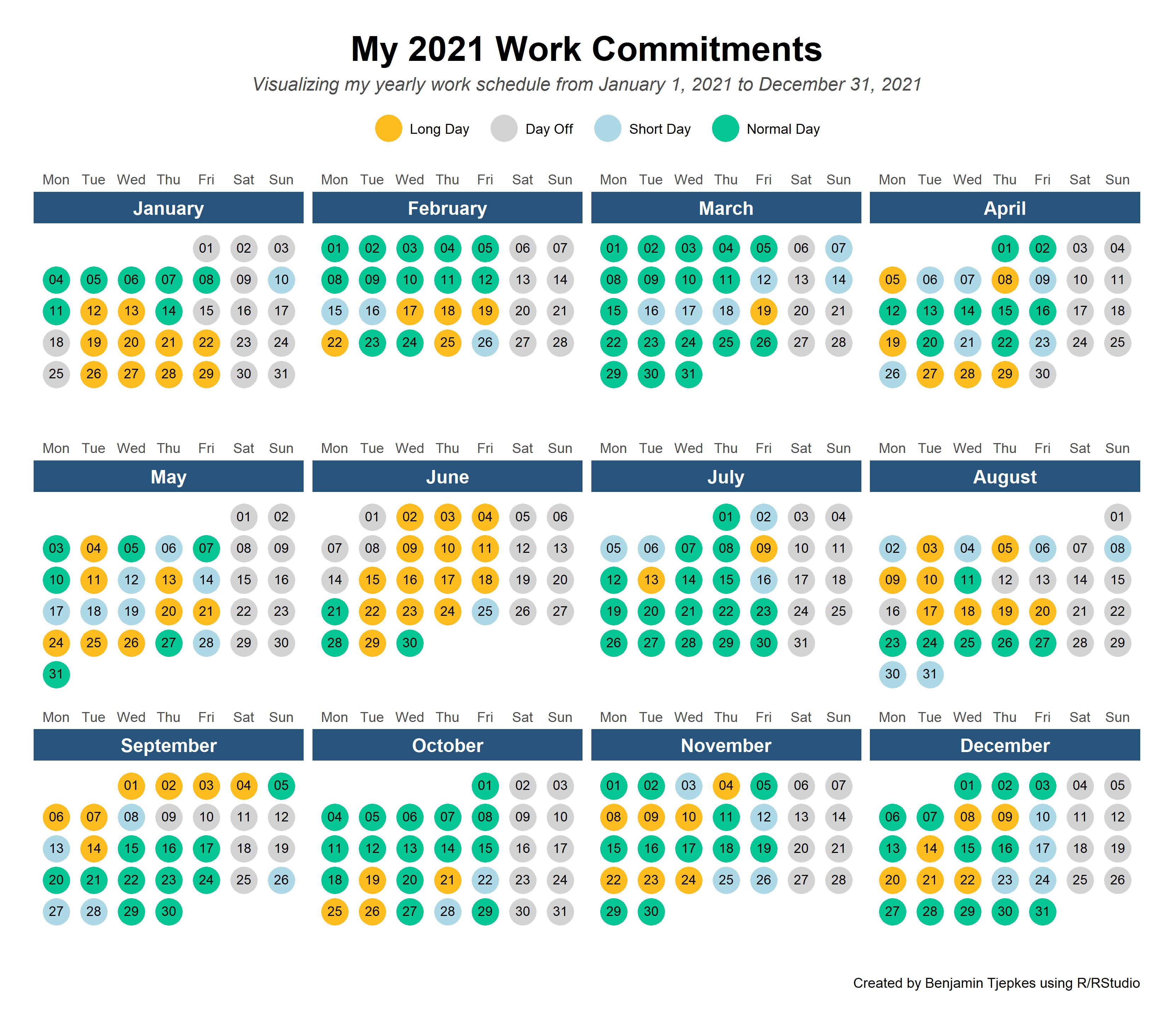
# LOAD PACKAGES ====

library(readxl)
library(tidyverse)
library(lubridate)

# LOAD DATA & WRANGLE ====

HourTracker_Tjepkes <- read_excel("HourTracker_Tjepkes.xlsx", 
                                  sheet = "Sheet2", col_types = c("date", "numeric", "numeric", "numeric", "numeric", "numeric", "numeric", "numeric", "numeric", "numeric",  "numeric", "numeric", "numeric", "numeric", "numeric", "numeric"))


HourTracker <- HourTracker_Tjepkes %>% 
  select(Date, `Total Hours`)

HourTracker$Date <- ymd(HourTracker$Date)


HourTracker_clean <- HourTracker %>% 
  mutate(Description = case_when(`Total Hours` == 0 ~ "Day Off",
                                  `Total Hours` > 8 ~ "Long Day",
                                 `Total Hours` == 8 ~ "Normal Day",
                                 `Total Hours` < 8 ~ "Short Day"))

unique_desc <- HourTracker_clean %>% 
                  distinct(Description) %>% 
                  pull(Description)

HourTracker_clean$Description <-factor(HourTracker_clean$Description,
                                       levels = unique_desc)


# CALENDAR FUNCTION ====

get_calendar <- function(start_date, end_date) {
  n_days <- interval(start_date,end_date)/days(1)
  date<-start_date + days(0:n_days)
  month_name<-format(date,"%B")
  month_num<-format(date,"%m")
  year<-format(date,"%Y")
  day_num<-format(date,'%d')
  day<-wday(date, label=TRUE)
  week_num<-strftime(date, format = "%V")
  cal<-data.frame(date, year, month_name, month_num, day_num, day, week_num)
  cal[cal$week_num>=52 & cal$month_num=="01","week_num"]=00
  
  week_month<-cal%>% 
    group_by(year,month_name, week_num)%>%
    summarise()%>%
    mutate(week_month_num=row_number())
  
  cal<-merge(cal, week_month, by=c("month_name"="month_name","week_num"="week_num","year"="year"))
  cal$month_name<-factor(cal$month_name, levels=c("January","February","March","April","May","June","July","August","September","October","November","December"))
  cal$day<-factor(cal$day, levels=c("Mon","Tue","Wed","Thu","Fri","Sat","Sun"))
  
  return(cal)
  
}

## create date range
start_date <- as.Date('2021-01-01')
end_date <- as.Date('2021-12-31')

## create calendar
cal<-get_calendar(start_date,end_date)

cal %>% View()


# JOIN CALENDAR & HOUR DATA ====

HourTracker_ForPlot <- left_join(cal,
                                 HourTracker_clean,
                                 by = c("date" = "Date"))

# CREATE PLOT

#custom color palette c('#26547c', '#ef476f', '#FFBC1F', '#05C793')
pal<-c('#FFBC1F', 'lightgray', 'lightblue', '#05C793')

#creating the plot
ggplot(HourTracker_ForPlot)+
  geom_tile(mapping = aes(x = day,
                          y=week_month_num),
            fill=NA) +
  
  geom_text(mapping = aes(x=day,
                          y=week_month_num,
                          label=day_num),
            color="black") +
  
  geom_point(data = HourTracker_ForPlot,
             mapping=aes(x=day,
                         y=week_month_num,
                         color = Description),
             size = 7.6) +
  
  geom_text(data = HourTracker_ForPlot,
            mapping=aes(x=day,
                        y=week_month_num,
                        label=day_num),
            color="black",
            nudge_y = 0.04,
            size = 3.0) +
  
  scale_y_reverse() +
  
  scale_color_manual(values = pal,
              guide = guide_legend(title.position  ="left",
                                   title.hjust = 0.5,
                                    title.vjust = 0.6,
                                  title="Type of Day:")) +

  
  scale_x_discrete(position = "top") +
  
  labs(y="", x= "", 
       title = 'My 2021 Work Commitments',
       subtitle = "Visualizing my yearly work schedule from January 1, 2021 to December 31, 2021",
       caption = "Created by Benjamin Tjepkes using R/RStudio") +
  
  facet_wrap(~month_name, scales = "free_x") +
  
  theme(
    legend.position = "top",
    axis.text.y = element_blank(),
    axis.ticks = element_blank(),
    panel.background = element_blank(),
    plot.title = element_text(hjust=0.5,
                              size=22,
                              face = "bold"),
    plot.subtitle=element_text(hjust = 0.5,
                               size = 12,
                               face = "italic",
                               color = "gray30"),
    legend.key = element_blank(),
    legend.title = element_blank(),
    legend.background = element_rect(),
    legend.spacing.x = unit(0.4, 'cm'),
    legend.text = element_text(margin = unit(c(0,0,0,-0.3), "cm")),
    strip.background = element_rect(fill = '#26547c'),
    strip.text = element_text(color = "white", face = "bold", size = 12),
    axis.text.x = element_text(hjust = 0.5),  # Align x-axis text to the top
    axis.title.x = element_blank(),  # Remove x-axis title
    
    plot.margin= unit(c(0.8,0.8,0.8,0.2), "cm")
  )

ggsave(filename = "calendar2.jpeg",
       plot = last_plot(),
       dpi = "retina")