# Optional install packages, if needed ----
# install.packages("tm")  # for text mining
# install.packages("SnowballC") # for text stemming
# install.packages("wordcloud") # word-cloud generator
# install.packages("RColorBrewer") # color palettes

# Load required packages, once installed ----
library("tm")
library("SnowballC")
library("wordcloud")
library("RColorBrewer")Introduction
This month (May), I wrapped up my first year as a graduate student which also brought my list of college courses up past 70! As the bags under my eyes can tell you, it has been a long road to this point, with much still left to go. I wanted to take some time to look back and reflect on the courses I have experienced in my higher education journey thus far by visualizing some course description data.
Why course descriptions?
College courses all come with a syllabus that lays out the course structure, objectives, and usually a brief official description. These descriptions detail the theory, methods, or general topics of each course and are officially registered with the Registrar. The main reason behind my decision to delve into these descriptions was finally completing my spreadsheet of courses over my academic career. Why did I bother with this? Well, I’m in the process of applying for various professional certifications, many of which require a record of all relevant courses taken. For example, I’ve been eyeing The Wildlife Society Certification Program for some time now.
Workflow - Word Cloud
The steps I took for this process came largely from this blog post, which was extremely helpful in understanding these text mining packages in R.
1. Data Processing
The first step we need to do is install and/or load all the required packages. This will include several new-to-me packages like tm and wordcloud along with some familiar ones like RColorBrewer.
2. Data Import
Next, we need to get our data into R and format everything as a tm::Corpus dataset that can be transformed in later steps.
# Load the text
text <- base::readLines(file.choose())

# Load the data as a corpus
docs <- tm::Corpus(VectorSource(text))
3. Data Wrangling
# Text transformation ----
toSpace <- content_transformer(function (x , pattern ) gsub(pattern, " ", x))
docs <- tm_map(docs, toSpace, "/")
docs <- tm_map(docs, toSpace, "@")
docs <- tm_map(docs, toSpace, "\\|")

# Text cleaning ----

# Convert the text to lower case
docs <- tm_map(docs, content_transformer(tolower))
# Remove numbers
docs <- tm_map(docs, removeNumbers)
# Remove english common stopwords
docs <- tm_map(docs, removeWords, stopwords("english"))
# Remove your own stop word
# specify your stopwords as a character vector
docs <- tm_map(docs, removeWords, c("course", "will"))
# Remove punctuations
docs <- tm_map(docs, removePunctuation)
# Eliminate extra white spaces
docs <- tm_map(docs, stripWhitespace)
4. Creating Matrix
# Build a Term-Document Matrix ----
dtm <- TermDocumentMatrix(docs)
m <- as.matrix(dtm)
v <- sort(rowSums(m),decreasing=TRUE)
d <- data.frame(word = names(v),freq=v)
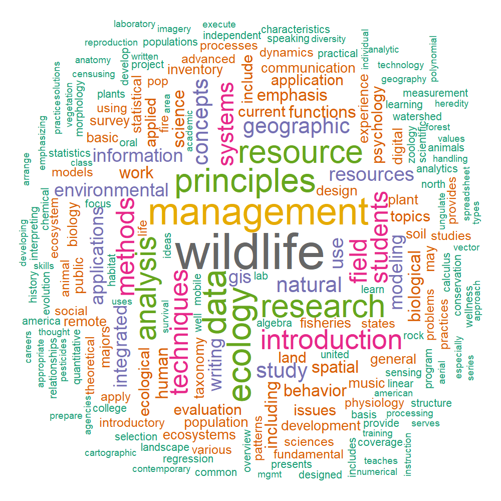
head(d, 10)5. Visualization
# Create and save word cloud
set.seed(1234)
grDevices::png(filename = "./word_plot.png",
               width = 1000,
               height = 1000,
               units = "px",
               res = 150)
wordcloud::wordcloud(words = d$word, freq = d$freq, min.freq = 1,
          max.words=200, random.order=FALSE, rot.per=0.35,
          colors=brewer.pal(8, "Dark2"))
grDevices::dev.off()
Citation
BibTeX citation:
@online{tjepkes2024,
  author = {Tjepkes, Benjamin},
  title = {Mining {Text} {From} {Course} {Descriptions}},
  date = {2024-05-21},
  url = {https://btjepkes.github.io/posts/text-mining-course-descriptions},
  langid = {en},
  abstract = {In this post, I describe a recent workflow that I ran on
    my college course descriptions to explore the most common words and
    word associations from my archive of college course.}
}
For attribution, please cite this work as:
Tjepkes, Benjamin. 2024. “Mining Text From Course
Descriptions.” May 21, 2024. https://btjepkes.github.io/posts/text-mining-course-descriptions.